R for UX Researchers Series: Article #7

Tutorial: User Sentiments in Reviews Using Text Mining

Summary: Learn how to use R and RStudio to perform sentiment analysis and uncover user sentiments from product reviews. This article covers data preparation, text mining techniques, analyzing sentiment scores, and creating data visualizations to support data-driven decision-making.

---

The Scenario

While leading user research at a SaaS company, the Director of UX came to me with this question:

"Can we figure out how users feel about our products using the data we already have, without having to set up a big survey or something like that?"

This question calls for a good old sentiment analysis. Sentiment analysis allows us to identify the emotional tone behind the text, which can reveal customers' opinions, feelings, and attitudes towards our products.

Using R and RStudio for this was the obvious choice because of their text mining capabilities and advanced visualization options. For something this complex, Excel or Google Sheets just wouldn't cut it.

Why Not Just Use Excel or Google Sheets?

To figure out user sentiments from product reviews, we need a toolset that can handle text mining and sentiment analysis. Here's why R and RStudio are the superior tools for this task:

1. Advanced Text Mining Capabilities: R has specialized packages like syuzhet for sentiment analysis and tm for text mining. Excel and Google Sheets don't have built-in capabilities for these complex analyses.

2. Handling Large and Complex Data: R manages and manipulates large datasets wayyyyyy better than Excel and Google Sheets.

3. Advanced Data Cleaning: R provides powerful functions for cleaning and preparing textual data. Tasks like removing punctuation, converting text to lower case, and eliminating stop words are straightforward in R but challenging in Excel or Google Sheets.

4. Reproducibility and Automation: R scripts automate the entire process, keeping things consistent and saving time when updating reports or applying them to different datasets.

5. Advanced Visualization: R can produce complex visualizations using packages like ggplot2 and wordcloud, which are not possible with Excel or Google Sheets.

Using R and RStudio for sentiment analysis allows us to gain deeper insights and provide more actionable recommendations based on user feedback. For this example, we’ll use an open-source Amazon Reviews dataset. While this isn't a perfect proxy for the Director of UX’s question above, you’ll be able to easily substitute your own data in place of this example.

Prerequisites

Before starting the tutorial, ensure you have completed the basic setup for R and RStudio as described in the "Getting Started with R & RStudio Tutorial." Additionally, if you are using Windows, you will need to install Rtools.

Step 1: Download the Dataset

First, download the Amazon Reviews Dataset on GitHub.

1. Visit the Amazon Reviews Dataset page on GitHub.

2. Click the Download raw file button in the top right of the Preview area to get the .csv file.

3. Save the downloaded file title amazon_reviews.csv on your computer.

✏️ NOTE: Make a note of the full path to the amazon_reviews.csv file on your computer. You'll need that path to import the datasets in step 5 below.

Step 2: Start a New RStudio Project

1. Open RStudio.

2. Go to File > New Project > New Directory > New Project.

3. Name your project (e.g., "Sentiment_Analysis_Reviews") and choose a location on your computer.

4. Click Create Project.

5. Set Up Your Project Structure: Within your new project directory folder on your computer, create a new folder and name it data.

6. Move the downloaded amazon_reviews.csv file into the new data folder that is in your project directory folder. This location is referred to as the files relative path.

You’ll know you have done this correctly when you see a new R file item and file folder titled data in the Files tab at the bottom right of the screen.

Step 3: Install Necessary Packages

Install the required packages by copying and pasting the code snippet below into the RStudio Console:

install.packages("tidyverse")
install.packages("tm")
install.packages("syuzhet")
install.packages("wordcloud")
install.packages("RColorBrewer")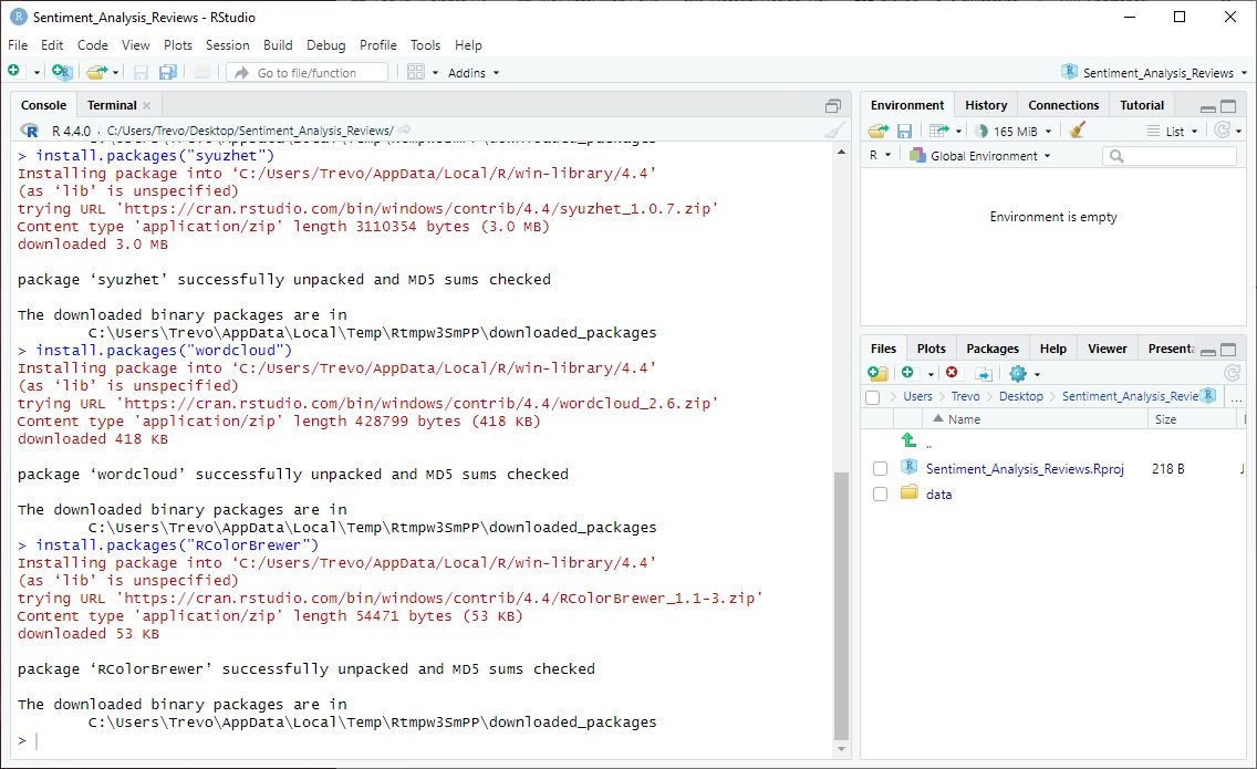

Step 4: Load the Libraries

Next, load the necessary libraries in your R script:

library(tidyverse)
library(tm)
library(syuzhet)
library(wordcloud)
library(RColorBrewer)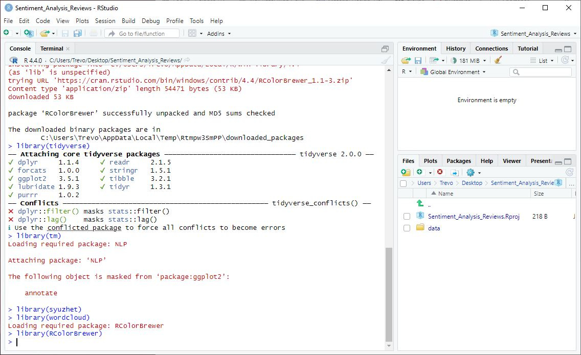

✏️ NOTE: Disregard the Conflicts section shown in the Console.

Step 5: Import the Dataset

Use a relative path to import the dataset.

# Import the dataset
file_path <- "path/to/your/dataset/amazon_reviews.csv"
reviews <- read_csv(file_path)

# View the first few rows of the dataset and check column names
head(reviews)
colnames(reviews)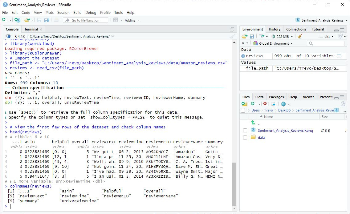

You’ll know you have done this correctly when you see new data items in the Environment tab at the top right of the screen.

✏️ NOTES:

• Replace "path/to/your/dataset" with the full paths on your own machine to amazon_reviews.csv file in the data folder.

• Viewing the first few rows of the dataset and checking column names using head(reviews) and colnames(reviews) is crucial for verifying that the dataset has been imported correctly and understanding its initial structure. This helps ensure that all necessary columns are present and allows you to get an overview of the data before proceeding with further analysis.

Step 6: Clean the Data

Let's prepare the data for analysis by handling missing values and ensuring the necessary columns are present. I’ll be writing an entire article about advanced data cleaning soon. Learn a little more about data cleaning in Article #5 in this series.

# Clean the data
reviews <- reviews %>%
  filter(!is.na(reviewText) & !is.na(overall))

# View the first few rows of the cleaned data
head(reviews)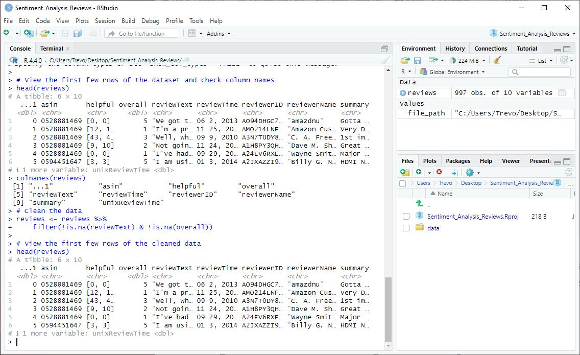

📘 Explanation: Cleaning the data involves filtering out rows with missing values in the reviewText and overall columns. Viewing the first few rows of the cleaned data using head(reviews) is important to confirm that the data cleaning process was successful and that any missing values have been appropriately handled. This step helps ensure the dataset is ready for accurate analysis, providing a quick overview of the cleaned data's structure.

Step 7: Perform Exploratory Data Analysis (EDA)

Now, let's explore the dataset to understand its structure and identify any patterns. Learn more about why I almost always run a EDA in my article R for UX Researchers Series: Article #2.

# Summary statistics
summary(reviews)

# Distribution of overall ratings
ggplot(reviews, aes(x = overall)) +
  geom_bar(fill = "steelblue", color = "black") +
  labs(title = "Distribution of Overall Ratings", x = "Rating", y = "Count") +
  theme_minimal()

# Word cloud of review text
review_corpus <- Corpus(VectorSource(reviews$reviewText))
review_corpus <- tm_map(review_corpus, content_transformer(tolower))
review_corpus <- tm_map(review_corpus, removePunctuation)
review_corpus <- tm_map(review_corpus, removeWords, stopwords("english"))
review_corpus <- tm_map(review_corpus, stripWhitespace)
wordcloud(review_corpus, max.words = 100, random.order = FALSE, colors = brewer.pal(8, "Dark2"))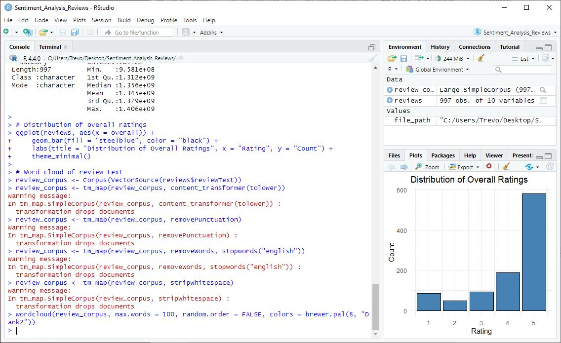

📘 Explanation: This EDA generates summary statistics and visualizations to help us understand the dataset. The distribution of overall ratings provides insight into the frequency of different ratings, while the word cloud visualizes the most common words in the review texts.

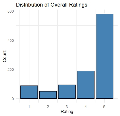
1. Summary Statistics

Overall Ratings:

• Mean: 4.129

• Median: 5.0

• Minimum: 1.0

• Maximum: 5.0

• 1st Quartile: 4.0

• 3rd Quartile: 5.0

2. Bar Chart

Sometimes a bar chart like this could be enough to satisfy your stakeholder, but we can do much better. Let’s really dive into this dataset.

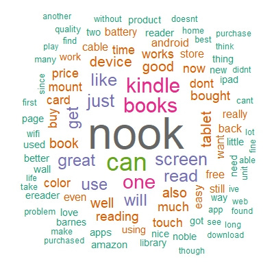
3. Word Cloud

Word clouds can be a visually appealing way to communicate the most frequent words in a dataset to stakeholders, making them useful for quickly highlighting key themes. However, they often lack the depth needed for thorough analysis. I rarely use them, but I've included one here for completeness.

This word cloud helps a bit but doesn't show context or tell us if mentions are positive or negative, so it's not very insightful.

Step 8: Perform Sentiment Analysis

Now let's perform the sentiment analysis on the review texts.

# Extract sentiment scores
sentiments <- get_nrc_sentiment(reviews$reviewText)

# Add sentiment scores to the original dataset
reviews <- cbind(reviews, sentiments)

# View the first few rows of the dataset with sentiment scores
head(reviews)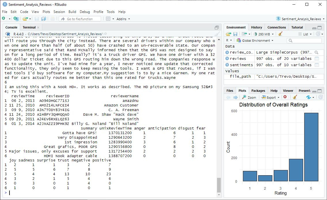

You’ll know you have done this correctly when you see your sentiment observations (obs.) in the Environment tab at the top right of the screen.

📘 Explanation: The get_nrc_sentiment function from the syuzhet package is used to extract sentiment scores from the review texts. These scores are then added to the original dataset for further analysis.

Step 9: Visualize Sentiment Analysis Results

Visualize the sentiment analysis results to understand the sentiment distribution in the reviews.

# Aggregate and visualize sentiment totals
sentiment_totals <- sentiments %>% 
  summarise(across(everything(), sum)) %>% 
  pivot_longer(cols = everything(), names_to = "sentiment", values_to = "total") %>% 
  arrange(desc(total))

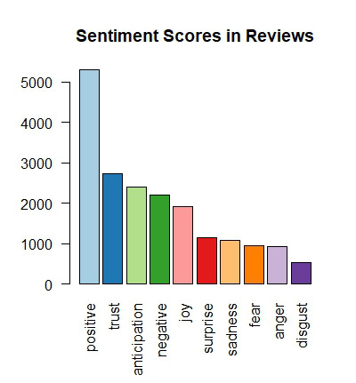
# Bar plot of sentiment scores
barplot(
  sentiment_totals$total,
  names.arg = sentiment_totals$sentiment,
  las = 2,
  col = brewer.pal(10, "Paired"),
  main = "Sentiment Scores in Reviews"
)

# Helper function to create a cleaned corpus
clean_corpus <- function(text_column) {
  corpus <- Corpus(VectorSource(text_column))
  corpus <- tm_map(corpus, content_transformer(tolower))
  corpus <- tm_map(corpus, removePunctuation)
  corpus <- tm_map(corpus, removeWords, stopwords("english"))
  corpus <- tm_map(corpus, stripWhitespace)
  return(corpus)
}

# Word cloud for positive words
positive_corpus <- reviews %>% 
  filter(positive > 0) %>% 
  pull(reviewText) %>% 
  clean_corpus()

wordcloud(
  positive_corpus,
  max.words = 100,
  random.order = FALSE,
  colors = brewer.pal(8, "Blues")
)

# Word cloud for negative words
negative_corpus <- reviews %>% 
  filter(negative > 0) %>% 
  pull(reviewText) %>% 
  clean_corpus()

wordcloud(
  negative_corpus,
  max.words = 100,
  random.order = FALSE,
  colors = brewer.pal(8, "Reds")
)

📘 Explanation: Explanation: In this step, we visualize the sentiment analysis results to uncover patterns in user feedback.

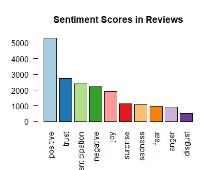
1. Bar Chart: The bar chart provides an overview of the total sentiment scores across all reviews, making it easy to identify which sentiments (e.g., joy, anger, trust) are most prevalent. This allows us to see the general emotional tone of the reviews at a glance.

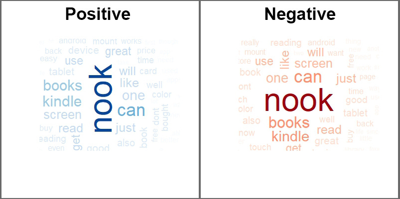
2. Word Clouds: The word clouds focus on the most common positive and negative words mentioned in reviews. By cleaning and filtering the text, we ensure the visualizations highlight the most relevant terms for each sentiment category. These word clouds are helpful for identifying key themes that users associate with their positive or negative experiences.

1. Bar Chart

This clearly shows the overall distribution of user emotions, making it easy to identify prevalent positive or negative feelings at a glance.

2. Word Clouds

Separating the word cloud into positive and negative sentiments still didn’t help to create meaningful data visualizations.

Although these show no meaningful differentiation, I decided to keep them in this tutorial to encourage you to run this analysis on your own data. It might reveal interesting insights specific to your context.

Step 10: Sentiment Score Distribution

Visualizing the distribution of sentiment scores can help us understand the overall spread and frequency of different sentiments in the reviews.

# Prepare sentiment scores for visualization
sentiment_scores <- sentiments %>% 
  pivot_longer(cols = everything(), names_to = "variable", values_to = "value")

# Density plot of sentiment scores
ggplot(sentiment_scores, aes(x = value, fill = variable)) +
  geom_density(alpha = 0.6) +  # Add smooth density curves
  scale_fill_brewer(palette = "Set3") +  # Use a visually distinct color palette
  labs(
    title = "Distribution of Sentiment Scores",
    x = "Sentiment Score",
    y = "Density"
  ) +
  xlim(0, 5) +  # Focus the x-axis to a meaningful range
  theme_minimal() +  # Apply a clean, minimal theme
  theme(
    legend.position = "top",  # Place the legend at the top for better readability
    legend.title = element_blank(),  # Remove the legend title
    axis.title.x = element_text(size = 12, face = "bold"),  # Emphasize x-axis title
    axis.title.y = element_text(size = 12, face = "bold"),  # Emphasize y-axis title
    plot.title = element_text(size = 14, face = "bold", hjust = 0.5)  # Center-align the plot title
  )

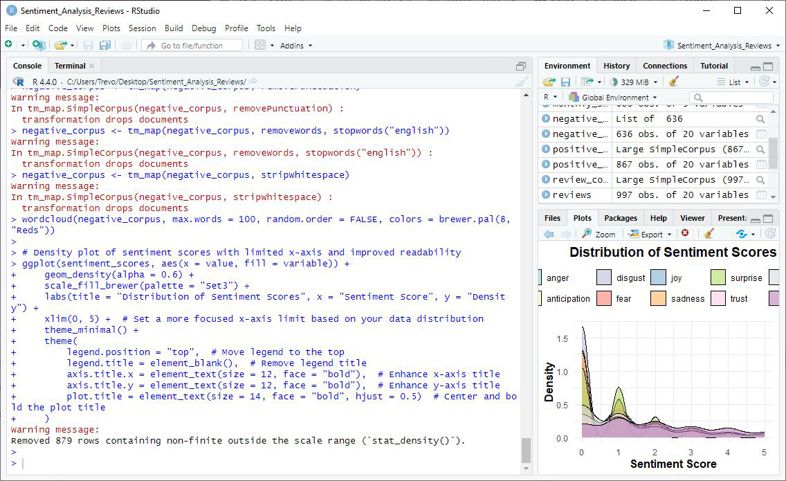
📘 Explanation: This density plot shows the distribution of individual sentiment scores across reviews, providing insight into the frequency and range of different sentiments. Before visualizing, we reshaped the data using the pivot_longer function, ensuring each sentiment category (e.g., joy, anger) and its corresponding scores are properly formatted for plotting.

The x-axis is limited to a more focused range of (0, 5), allowing us to ‘zoom in’ on the bulk of the data and ignore extreme outliers that might obscure meaningful patterns. This adjustment makes the plot more interpretable and actionable.

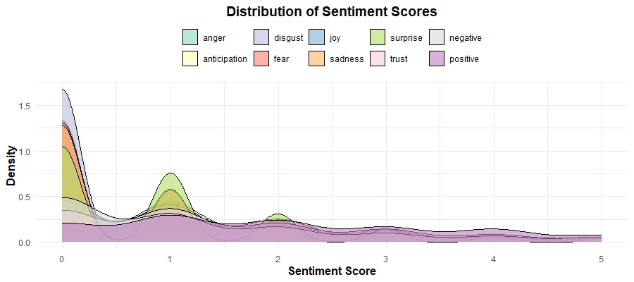
This plot is critical for understanding how users' emotions are distributed across different sentiment categories. Peaks in the density plot indicate common sentiment scores. For example:

• Positive sentiments, such as joy and trust, have a notable presence, indicating that many users hold a generally favorable opinion of the products.

• Negative sentiments, such as anger and disgust, while less frequent, highlight areas for potential improvement.

Step 11: Sentiment by Rating

Comparing the average sentiment scores across different overall ratings can reveal how sentiments relate to product ratings.

# Calculate average sentiment scores by rating
avg_sentiment_by_rating <- reviews %>%
  group_by(overall) %>%
  summarize(across(colnames(sentiments), mean, na.rm = TRUE))

# Reshape the data frame for plotting
avg_sentiment_by_rating_melted <- avg_sentiment_by_rating %>% 
  pivot_longer(cols = -overall, names_to = "variable", values_to = "value")

# Bar plot of average sentiment scores by rating
ggplot(avg_sentiment_by_rating_melted, aes(x = factor(overall), y = value, fill = variable)) +
  geom_bar(stat = "identity", position = "dodge") +
  scale_fill_brewer(palette = "Set3") +
  labs(
    title = "Average Sentiment Scores by Rating",
    x = "Overall Rating",
    y = "Average Sentiment Score"
  ) +
  theme_minimal()

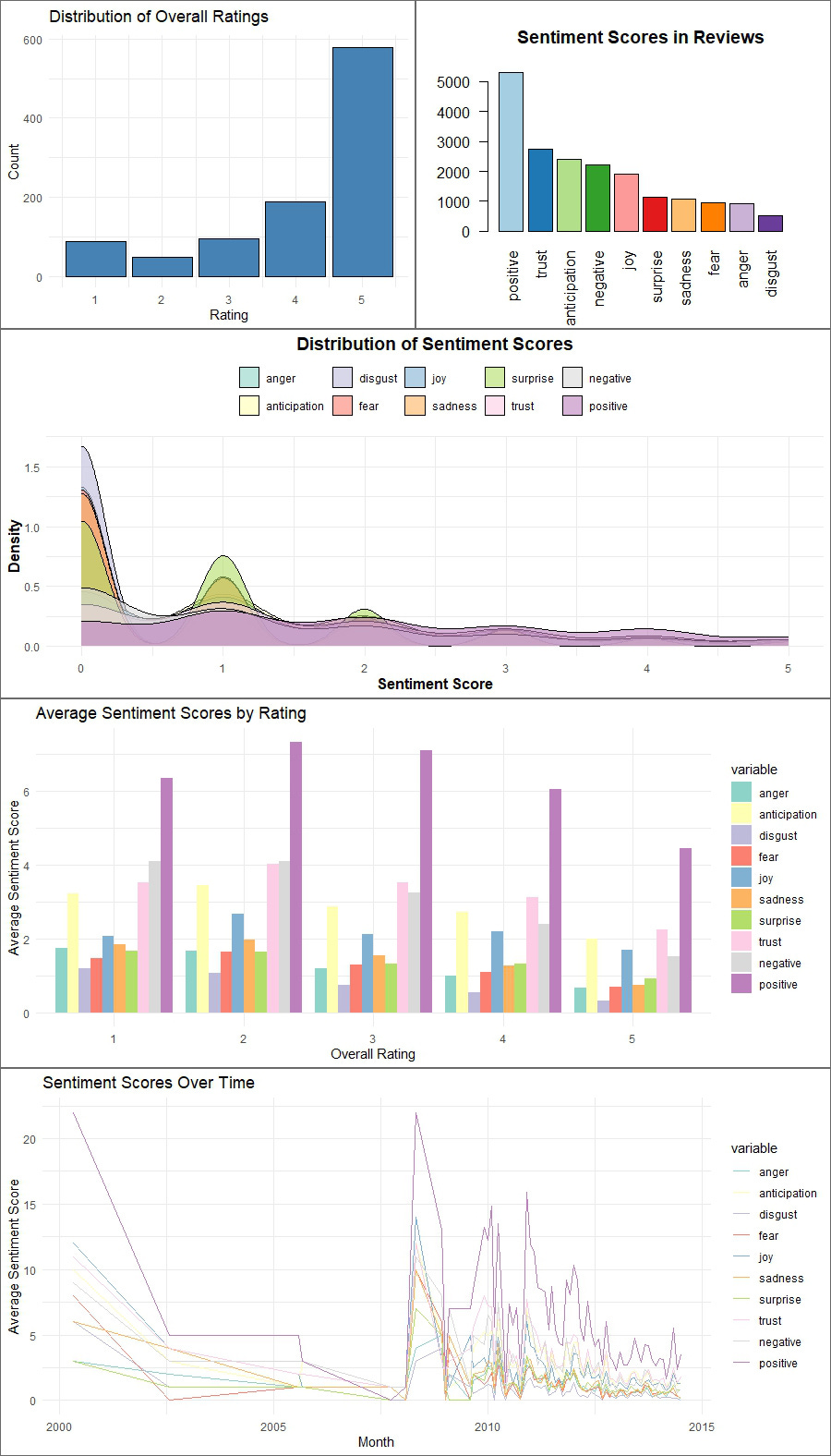
📘 Explanation: This bar plot compares the average sentiment scores for different overall ratings, providing insight into how sentiment varies with user ratings.

Before creating the visualization, we used pivot_longer to reshape the data. This step organizes sentiment categories (e.g., joy, trust, anger) into a single column, allowing the scores to be visualized effectively. Reshaping the data ensures that each sentiment type is grouped and displayed correctly in the bar plot.

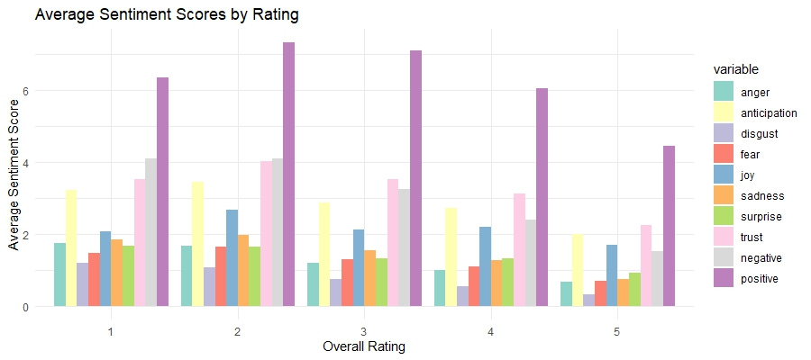
The bars illustrate the relationship between user ratings and their associated emotions:

• Higher Ratings (4 and 5 stars): These ratings have higher scores for positive sentiments such as joy and trust, reflecting satisfaction and approval from users.

• Lower Ratings (1 and 2 stars): These ratings are associated with higher scores for negative sentiments such as anger and disgust, indicating areas of dissatisfaction.

This visualization helps us pinpoint which sentiments are most closely tied to different levels of user satisfaction. By identifying strengths (e.g., positive emotions for higher ratings) and areas for improvement (e.g., negative sentiments for lower ratings), we can better understand user feedback and prioritize targeted actions to enhance the product experience.

Step 12: Time Series Analysis

Comparing the average sentiment scores across different overall ratings can reveal how sentiments relate to product ratings.

# Convert reviewTime to Date format
reviews$reviewTime <- as.Date(reviews$reviewTime, format = "%m %d, %Y")

# Aggregate sentiment scores by month
monthly_sentiment <- reviews %>%
  group_by(month = floor_date(reviewTime, "month")) %>%
  summarize(across(colnames(sentiments), mean, na.rm = TRUE))

# Melt the data frame for plotting
monthly_sentiment_melted <- melt(monthly_sentiment, id.vars = "month")

# Line plot of sentiment scores over time
ggplot(monthly_sentiment_melted, aes(x = month, y = value, color = variable)) +
  geom_line() +
  scale_color_brewer(palette = "Set3") +
  labs(title = "Sentiment Scores Over Time", x = "Month", y = "Average Sentiment Score") +
  theme_minimal()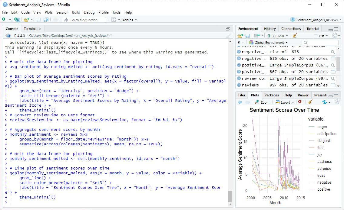

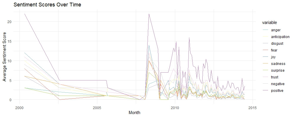
📘 Explanation: This line plot shows how sentiment scores have changed over time, revealing trends and patterns in user sentiment.

These lines show the fluctuation of sentiment scores over time, highlighting trends and shifts in user emotions. For instance, we can observe periods where positive sentiments like joy and trust peaked, possibly indicating successful product updates or positive user experiences. Conversely, spikes in negative sentiments such as anger and disgust may point to times when users faced issues. This visualization allows us to track the impact of changes and events on user sentiment, helping us understand and respond to user needs more effectively.

Interpreting the Data

Now that we've performed sentiment analysis and visualized the results, let's make sense of the findings. I’ll focus on these five visuals that tell the best story found in the data.

1. Distribution of Overall Ratings

   The bar chart of overall ratings shows that the majority of reviews are positive, with 4 and 5-star ratings being the most common. This clearly shows that users have a favorable view of the products.

   

2. Sentiment Distribution in Reviews

   The bar chart of sentiment scores reveals the overall distribution of different sentiments in the reviews. Here are some specific things I noticed in this plot:

   

   • Prominent Positive Sentiments: The most prominent sentiment is "positive," suggesting users generally have a favorable view of the products.

   • Negative Sentiments: Negative sentiments like "disgust," "fear," and "anger" are less frequent but still present, signaling areas for potential improvement.

   • Joy and Surprise: While positive sentiments like "joy" and "surprise" are present, the "negative" sentiment outnumbers both, indicating significant negative experiences that need to be addressed to enhance overall user satisfaction.

3. Sentiment Score Distribution

   This density plot of sentiment scores provides a detailed view of the frequency and range of different sentiments. This suggests that while extreme sentiments are less common, there is a wide variety of mild to moderate sentiments expressed in the reviews. Here are some specific things I noticed in this plot:

   

   Remember, we focused on a limited range (0-5) to better understand the bulk of the data, revealing that most sentiment scores are clustered towards the lower end, with a sharp peak around zero.

   • Dominance of Low Scores: The sharp peak around zero indicates that most reviews contain a mix of low-intensity sentiments, which might suggest that users often express mild feelings rather than strong emotions in their reviews.

   • Presence of Negative Sentiments: There are noticeable peaks for sentiments like "negative" and "fear" around the lower end of the scale. This indicates that, even though these sentiments are less frequent overall, they are still significant and should be looked into further.

   • Recurrent Patterns: There are recurring patterns of sentiment fluctuations. Periodic rises in positive sentiments might correspond with product updates or successful marketing efforts, while dips could reflect recurring issues or negative feedback cycles.

4. Sentiment by Rating

   These bar charts comparing average sentiment scores by rating shows how sentiments vary with overall user ratings. Higher ratings (4 and 5 stars) are associated with positive sentiments like "joy" and "trust," while lower ratings (1 and 2 stars) correspond to negative sentiments such as "anger" and "disgust." This relationship between sentiment and rating confirms that sentiment analysis can effectively capture the emotional tone of user feedback, aligning with their overall satisfaction. Here are some specific things I noticed in this plot:

   

   • Higher Anticipation in Mid-Ratings: Sentiment scores for "anticipation" are relatively high for 3-star ratings, suggesting that users who gave an average rating might still have hopeful expectations or mixed feelings about the product.

   • Negative Sentiments Even in High Ratings: Even in higher ratings (4 and 5 stars), there are notable levels of negative sentiments like "sadness" and "fear." This indicates that while users are generally satisfied, there are still aspects of the product that might cause concern or disappointment.

   • Low Surprise Across Ratings: The sentiment "surprise" has low scores across all ratings, indicating that the products generally meet user expectations without offering unexpected positive or negative experiences. This could be an area to explore improving overall user experience.

5. Sentiment Scores Over Time

   The line plot of sentiment scores over time reveals trends and patterns in user sentiment. For example, if there is a noticeable increase in positive sentiments like "joy" and "trust" over a specific period, it may indicate the successful implementation of product improvements or effective marketing campaigns. Conversely, a rise in negative sentiments like "anger" and "disgust" could signal emerging issues that need to be addressed promptly. Here are some specific things I noticed in this plot:

   

   • Big Dips and Big Spikes: Check out the drop in positive sentiments, such as "joy" and "trust," around 2005. At the same time, there is a big spike in negative sentiments like "anger" and "disgust." This would prompt me to further investigate the factors that might have affected user perception during that critical period. There could be some valuable “lessons learned” insights there.

   • Stable Sentiments Post-2007: After 2007, sentiments stabilize with less volatility. This suggests that the company might have resolved major issues, leading to more consistent user experiences and satisfaction levels.

   • Recurrent Patterns: There are recurring patterns of sentiment fluctuations. Periodic rises in positive sentiments might correspond with product updates or successful marketing efforts, while dips could reflect recurring issues or negative feedback cycles.

   • Low Frequency of Extreme Sentiments: The low frequency of extreme positive and negative sentiments after 2007 indicates that most reviews fall within a moderate range, suggesting a balanced user experience with fewer extreme reactions.

Each of these visualizations offers a unique perspective on user feedback, but together they provide a comprehensive understanding of user sentiment.

By looking at these visuals collectively, we gain a holistic view of user sentiment, enabling us to identify both strengths to build upon and areas needing attention.

Here are 4 things I noticed when looking at all the plots together:

1. Context for Negative Sentiments: The "Sentiment Distribution in Reviews" bar chart shows the presence of negative sentiments such as "disgust," "fear," and "anger." When cross-referenced with the "Sentiment Scores Over Time" line plot, we can identify specific periods (like around 2005) when these negative sentiments spiked, suggesting potential historical issues that impacted user perception.

2. Long-Term Sentiment Stability: The "Sentiment Scores Over Time" line plot shows a stabilization in sentiments post-2007. Cross-referencing this with the "Sentiment Score Distribution" density plot, we observe a clustering of mild to moderate sentiments, suggesting that while extreme sentiments have become less frequent, the overall user sentiment has balanced out over time.

3. Specific Sentiment Peaks: The "Distribution of Sentiment Scores" density plot highlights peaks in sentiments like "anticipation" and "negative." By correlating these findings with the "Average Sentiment Scores by Rating" plot, we can infer that users experiencing "anticipation" might have higher expectations that lead to mixed or negative reviews if unmet.

4. Identifying Improvement Areas: The "Sentiment Distribution in Reviews" bar chart shows fewer negative sentiments, but their presence is significant. By combining this with the "Sentiment Scores Over Time" line plot, we can track when these sentiments were most prevalent and use this insight to identify specific periods or product updates that might need further investigation to understand and address user dissatisfaction.

Actionable Insights

Based on the sentiment analysis and data interpretation, here are some actionable insights for the Director of UX:

1. Further Enhance Positive Aspects:

   • Double down on the things that users loved, such as "usability" and "quality," which appeared many times in the reviews, and make sure these aspects don't slip over time.

   • Highlight these positive aspects in marketing and communication efforts.

2. Address Negative Feedback:

   • Investigate the issues mentioned in negative reviews, such as specific problems and disappointments.

   • Develop strategies to address these pain points, whether through product improvements, better customer support, or clearer user instructions.

3. Monitor Trends:

   • Continuously monitor sentiment scores over time to identify emerging trends and respond proactively.

   • Use this data to guide future product development and customer engagement strategies.

4. Segment-Specific Insights:

   • Consider segmenting the data further by product lines, user demographics, or other relevant factors to gain more targeted insights.

   • Tailor your strategies to address the specific needs and preferences of different user segments.

Conclusion

Well that’s it. You finished another tutorial! I want you to imagine how powerful this data would be when reported to the Director of UX, and how good you would look by recommending further investigation into the insights that could be gained by segmenting the data by product lines, user demographics, or other factors.

This is when UX research shines the most—when you can answer questions your stakeholders didn't even know they needed to ask.

Once you do this kind of deep work, the questions of value and “seat at the table” just go away. There's no need to fight any type of political battle like many online UX influencers seem to recommend. Just old-school, merit-based value-adding. It does the trick every time. hahahaha.

Feedback

I hope you found this tutorial on sentiment analysis using R and RStudio helpful. If you have any questions, suggestions, or feedback, please feel free to reach out. Your input is invaluable as I continue to create content to help you leverage data in UX research. Thank you for following along!

---